An important feature of the Excel spreadsheet program is that it allows you to create formulas that will automatically calculate results. Without formulas, a spreadsheet is not much more than a large table for displaying text.
Formulas
A formula is an equation that makes calculations based on the data in your spreadsheet. Formulas are entered into a cell in your worksheet. They must begin with an equal sign, followed by the addresses of the cells that will be calculated upon, with an appropriate operand placed in between. Once the formula is typed into the cell, the calculation executes immediately. The formula appears in the formula bar. ![]()
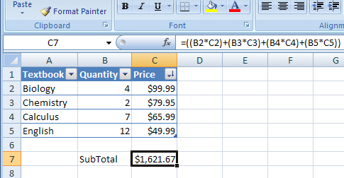
In the example below, a formula has been created for calculating the subtotal of a number of textbooks. This formula multiplies the quantity and price of each textbook, and then adds the totals to give the combined cost of all books.
Linking Worksheets
You can create a formula that uses data from two different worksheets. This can be done within the same workbook or across different workbooks. The base formula is written as “sheetname!celladdress” when linking cells from worksheets within the same workbook. The base formula is written as “[workbookname.xlsx]sheetname!celladdress” when linking cells from different workbooks. For example, the value of cell A1 in Worksheet 1 and cell A2 in Worksheet 2 can be added using the formula “=A1+Sheet2!A2”. Similarly, suppose Worksheet 1 was in a workbook named Book1.xlsx, and Worksheet 2 was in a workbook called Book2.xlsx, the same cells could be added using the formula “=[Book1.xlsx]Sheet1!$A$1+A2”. This formula would of course be entered inside Sheet2 of Book2.xlsx.
Relative, Absolute, and Mixed Referencing
Relative referencing is the practice of calling cells by just their column and row labels (such as “A1”). When a formula contains relative referencing and it is copied from one cell to another, Excel does not create an exact copy of the formula. It will change cell addresses relative to the row and column they are moved to. For example, if a simple addition formula in cell C1 “=(A1+B1)” is copied to cell C2, the formula would change to “=(A2+B2)” to reflect the new row.
To prevent this from happening, cells must be called by absolute referencing. This is accomplished by placing dollar signs “$” within the cell addresses in the formula. Continuing the previous example, if the formula in cell C1 reads “=($A$1+$B$1)”, the value of cell C2 will be the sum of cells A1 and B1. Both the column and row of both cells are absolute and will not change when copied. Mixed referencing can also be used where the row OR column is fixed, but not both. For example, in the formula “=(A$1+$B2)”, the row of cell A1 is fixed and the column of cell B2 is fixed.
Basic Functions
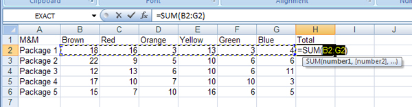
Functions can be a more efficient way of performing mathematical operations than formulas. For example, if you wanted to add the values of cells D1 through D10, you would type the formula “=D1+D2+D3+D4+D5+D6+D7+D8+D9+D10”. A shorter way would be to use the SUM function and simply type “=SUM(D1:D10)”. Several other function commands and examples of functions are given in the table below:
| Function | Example | Description |
|---|---|---|
| SUM | =SUM(A1:A100) | Finds the sum of cells A1 through A100 |
| AVERAGE | =AVERAGE(B1:B10) | Finds the average of cells B1 through B10 |
| MAX | =MAX(C1:C100) | Returns the highest number from cells C1 through C100 |
| MIN | =MIN(D1:D100) | Returns the lowest number from cells D1 through D100 |
| SQRT | =SQRT(D10) | Finds the square root of the value in cell D10 |
| TODAY | =TODAY() | Returns the current date (leave the parentheses empty) |
The Function Wizard
Excel has menus of other available functions that can be accessed using the Function Wizard. To select a function using the Function Wizard:
- StepsActions
- Click the cell where the function will be placed.
- In the Function Library group, click the Formulas tab. The Insert Function dialog box opens.
Note: The same Insert Function button can be found at all times right to the left of the Formula Bar and to the right of the Name Box.
- StepsActions
- From the Category drop-down menu, select a function category.
- From the Select a function menu, select a function type. A description and example of the function appears below the menu.
- Click OK. The Function Arguments dialog box opens.
- Choose the cells that will be included in the function.
- When all the cell values for the function have been entered, click OK.
Autosum
Use the Autosum function to add the contents of a cluster of adjacent cells.
- StepsActions
- Highlight the group of cells that will be summed (cells B2 through G2 in this example).
- Click the Formulas tab.
- Click Autosum.